Under the weather: Stochastic variance in VRE returns

What reference years can't capture

AEMO's Integrated System Plan, for example, relies on a set of historical reference years to represent the range of possible conditions. This preserves real-world correlations between demand, wind and solar across regions, but is constrained to combinations of conditions that have actually occurred. Unusual or novel weather combinations that are statistically plausible but have not yet been observed fall outside the modelled range.

Modelling the full distribution

Our approach generated 500 synthetic but physically realistic scenarios using a Monte Carlo simulation framework, with correlations preserved across asset-level wind output, asset-level solar output, and statewide demand. The result is a distribution of outcomes that includes novel combinations of conditions that are statistically plausible but have never been observed before.

Weather risk is not equal across technologies

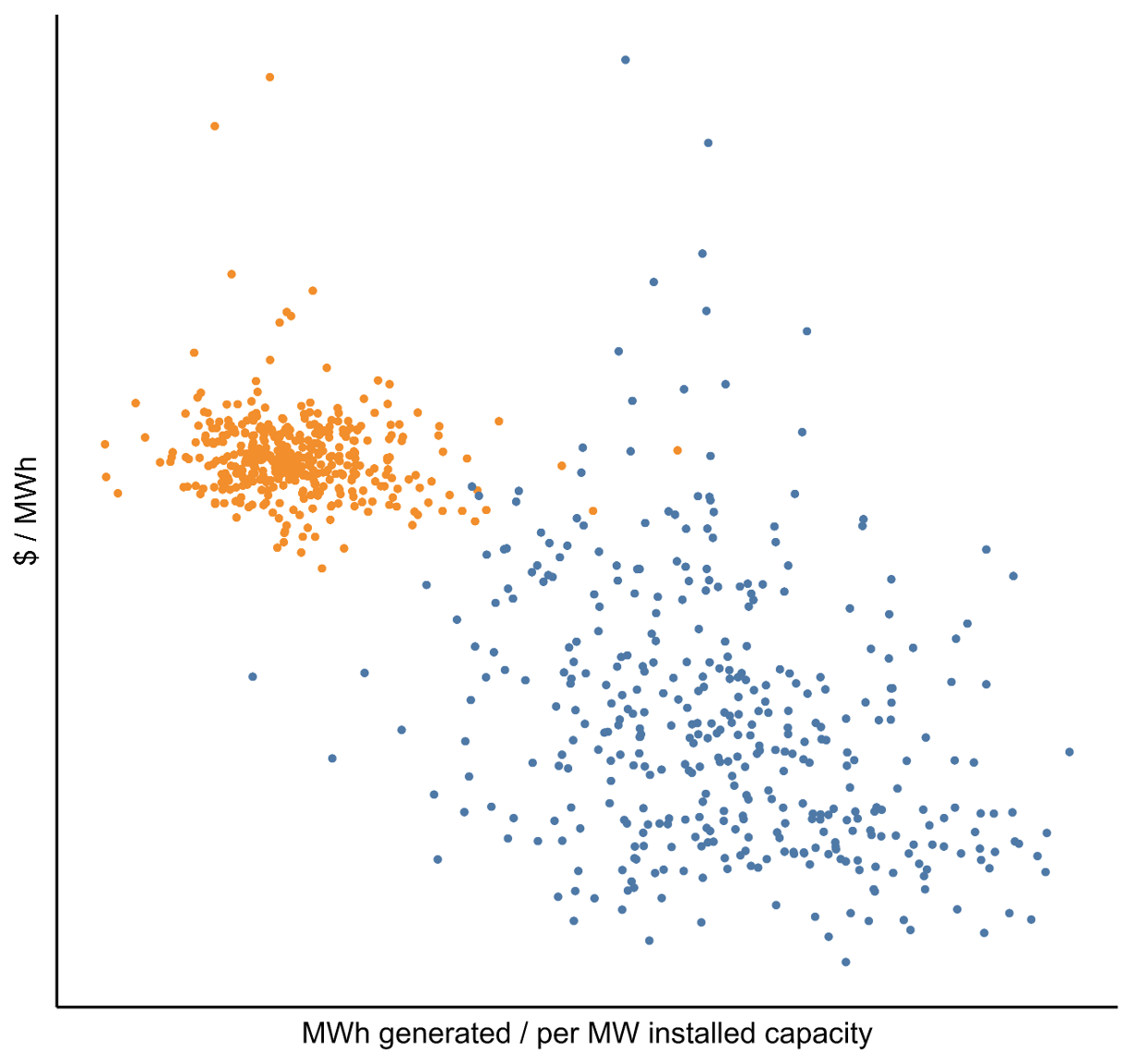
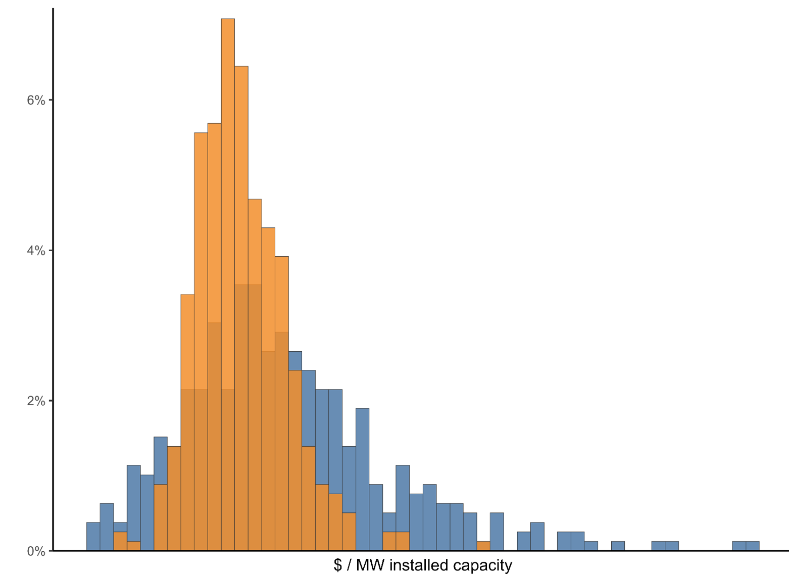
Chart 1 plots each of 500 simulated Januaries for a solar farm in Queensland and a wind farm in South Australia. The contrast is immediate:

• Wind outcomes are far more dispersed. Revenue varies widely across simulations, reflecting the day-to-day unpredictability of wind resources.
• Solar outcomes cluster more tightly. Solar follows a more predictable diurnal pattern, which constrains the range of possible generation and revenue outcomes.

The width of each distribution shows the revenue risk an asset owner faces from weather variability alone, before any consideration of other typical risks like market, network congestion or policy risks.

Chart 1: Generation and price spread (left) | Distribution of revenue (right) · QLD solar and SA wind, 500 simulations, January 2026

Source: BBA Stochastic Probability Model; BBA Power Model. Captured $/MWh are outputs from an SRMC-only dispatch model. Get in touch to discuss how we integrate more sophisticated bidding and pricing assumptions.

What this means for asset owners

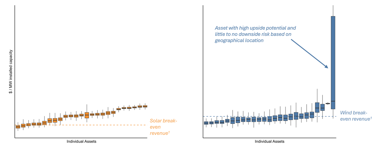
Chart 2 extends this to 25 randomly selected assets across the NEM. Even within each technology, there is substantial variation in both the level and spread of simulated revenue. Some solar assets show tight distributions well above their break-even revenue threshold, suggesting strong economics regardless of the weather scenario. Wind assets show a wider spread, with certain assets facing significant downside exposure in low-wind scenarios while others carry large upside potential.

Chart 2: Simulated solar and wind revenue for 25 randomly selected assets, January 2026

Source: BBA Stochastic Probability Model; BBA Power Model. Captured $/MWh are outputs from an SRMC-only dispatch model. Get in touch to discuss how we integrate more sophisticated bidding and pricing assumptions.

For asset owners and investors working from a single forecast, a point estimate says nothing about the range of outcomes around it. An asset with a strong central case can still carry significant downside exposure in tail scenarios, and that exposure varies substantially by location, technology, and resource quality.

Understanding that distribution is what allows for more informed decisions on asset selection, project financing, and portfolio construction. As the renewable fleet grows and weather-driven revenue risk becomes a more significant factor in project economics, the ability to model that risk with greater precision will only become more valuable.

References and methodology